Chapter 2 Models for Limited Dependent Variables
2.1 Logit
Open the 2008 Cooperative Congressional Election Study dataset and recode some of the variables so that they will be appropriately coded:
use http://people.umass.edu/schaffne/cces08.dta
recode cc316c 2=0 3=., gen(stemcell)
recode cc307 2=-1 3=0 4/5=., gen(pid)
recode v243 6=., gen(ideology)
ren v213 education
The logit command in Stata works similarly to the regress command. You begin your line with logit and then list the dependent variable followed by your independent variables. An alternative to logit is probit, which works similarly, but assumes a different variance.
logit stemcell pid ideology education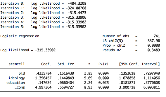
It is important to keep in mind that the coefficients are not easily interpreted in the way that OLS coefficients are. You can ask Stata to give you odds ratios instead of coefficients by adding , or to the end of your logit command.
logit stemcell pid ideology education, or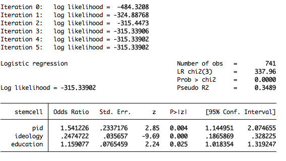
You can interpret the odds ratios a bit more easily. For example, you could interpret the odds ratio on education to mean that for each additional unit increase on the scale education, an individual’s odds of supporting stem cell research are 1.16 times greater. Or, perhaps slightly more intuitively, for each additional education category, an individual’s odds of supporting stem cell research increase by 16%. When you ask for odds ratios you don’t get an intercept, since the intercept doesn’t have an odds ratio.
Now, let’s return to interpreting those coefficients. While odds ratios are fairly easy to calculate, they probably aren’t the best way to talk about the effects of the coefficients. More ideal and easy to understand are predicted probabilities. You can generate and plot these using the margins and marginsplot commands.
First, margins will return a list of predicted probabilities under different conditions that you can specify. For example, if you wanted to know the probability that an individual who is “very liberal” on the ideology measure and average on the other covariates would support funding for stem cell research you could use this command:
margins, at(ideology=1) atmeans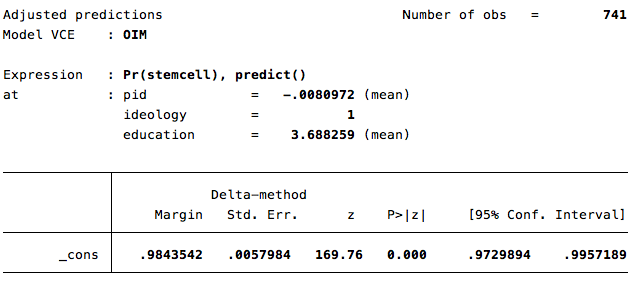
Note that there is a .98 probability that this individual would support funding for stem cell research. Also note that the command gives you a 95% confidence interval for that prediction.
Now what if you want to plot the predicted probabilities across all values of ideology? To do this, you first need to ask for those probabilities using the margins command. Then you can follow that up with the marginsplot command to graph them.
margins, at(ideology=(1(1)5)) atmeansNote that the command above asks for predictions of support for stem cell research at every value between 1 and 5 in 1 point increments (this is the clause ideology=(1(1)5)).
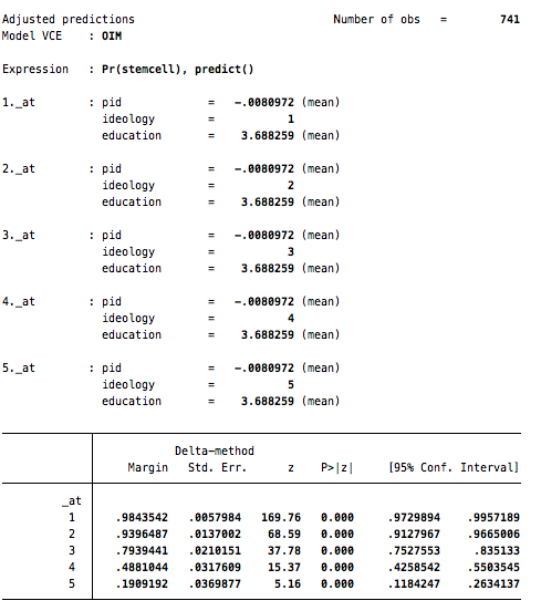
Now, you can use the marginsplot command to plot these predicted probabilities…
marginsplot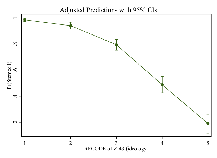
And now if we want to clean this graph up a bit, we can do that by adding some options to re-name the axis and graph titles:
marginsplot, ytitle("Prob. of supporting funding for stem cell research") xtitle("Ideology") title("Effect of Ideology on Stem Cell Support")
2.2 Ordinal Logit
An ordinal logit model is used when you have a dependent variable that takes on more than two categories and those categories are ordered. For example, Likert scales, common in survey research, are ordered dependent variables.
The command to estimate an ordinal logit model in Stata is ologit.
In the 2008 CCES dataset, there is a question asking respondents their views on Affirmative Action policies (cc313). Respondents can indicate their support for such policies on a four point scale, ranging from 1 (“Strongly support”) to 4 (“Strongly oppose”). One could collapse these categories into “support” or “oppose,” but why throw away detail about the strength of support?
To estimate an ordinal logit model on this question, you could use the following command:
ologit cc313 ideology pid education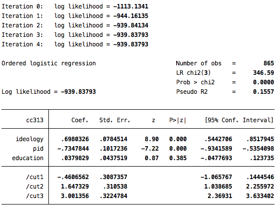
The coefficients in this output are estimating the effect of a one unit increase in each independent variable on the log odds of moving to a higher category on the scale of the dependent variable. These can be converted to odds ratios using the same or option noted above.
Predicted probablities can be created using the marginsplot command. Following the process outlined below for mlogit will work with ologit as well (to create predicted probabilities for each outcome category).
2.3 Multinomial Logit
For cases when the dependent variable has unordered categories, we use multinomial logit. In Stata, you would use the mlogit command to implement this type of model. Let’s use variable cc309 as our dependent variable. That variable asks respondents what they would most want to do to balance the federal budget – cut defense spending (1), cut domestic spending (2), or raise taxes (3). Let’s use the same set of independent variables.
mlogit cc309 ideology pid education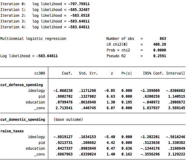
Each coefficient and statistical test above is calculated in relation to the base category (cut domestic spending). So, the coefficients are telling you whether a coefficient means there is a significant difference between the odds of choosing the category relative to the base category, but not whether there is a significant difference across other categories.
As with the logit model, you can again create predicted probabilities and plots to help look at the size of the effects.
margins, at(ideology=(1(1)5)) atmeans
marginsplot, ytitle("Probability"") xtitle("Ideology"") 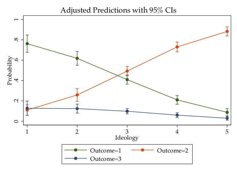
Let’s clean this up a bit to make things clearer. In particular, let’s label the legend better by adding an option to label each key in the legend. I’m also going to get rid of the title by specifying a blank title:
marginsplot, ytitle("Probability"") xtitle("Ideology") title("") legend(order(1 "Cut defense"" 2 "Cut domestic"" 3 "Raise taxes"")) 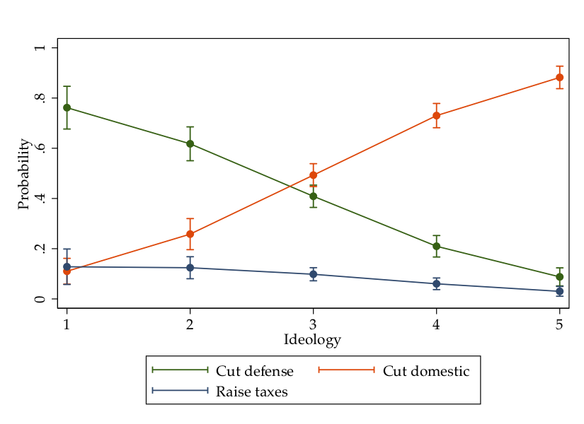
The graphic shows that most of the effect of ideology occurs in choosing between the “cut defense” and “cut domestic” categories. Almost everyone, regardless of ideology, prefers to not raise taxes.