Chapter 8 Panel Data
We will use the 2010-2014 CCES Panel Data as an example to demonstrate some panel analysis techniques. You may download the survey from here.
8.1 Reshaping Data
The CCES data comes in “wide” format. That means that each row is an individual and their responses for each year of the survey are recorded across the dataset in columns. For example, the variable CC10_308a is the individual’s approval of President Obama in 2010, CC12_308a is the approval of Obama in 2012, and CC14_308a is the value of approval for 2014.
While there may be some value to having data appear in this format, it is necessary to change to “long” format in order to conduct panel analyses in Stata. Long format means that there is a separate observation for each individual in each year. Thus, what you would end up with for this panel dataset is three observations for each respondent (2010, 2012, and 2014) with one variable for each question that was asked in each of those years. In other words, instead of having CC10_308a, CC12_308a, and CC14_308a, you would want just a single CC_308a. You would then have a caseid variable that is unique to each respondent, and a year variable that indicates which year each variable applies to.
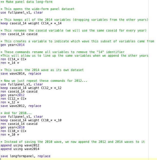
Once we understand some of the re-naming conventions, it is not particulalry difficult to re-shape the dataset so that it works in this form. The do-file below shows how we would do this with the wide-form panel data. The basic gist is that we would be subsetting the wide-form dataset into three different datasets: one for each wave (or year). We then rename the variables so that they will have the same variable names in each year (e.g. CC_308a instead of CC10_308a, CC12_308a, and CC14_308a).

Once you have your data set up in long form, you can tell Stata that it is in panel format. To do this, you use the xtset command and then follow that command first with the variable indicating each unique respondent and the variable indicating each time period.
xtset caseid yearHowever, in this case we want to specify to Stata that the time periods in our analysis happen every two years rather than every year. Thus, we can include an additional option to the above command to make this clear:
xtset caseid year, delta(2)8.2 Panel Analysis
Now that we have xtset the data, we can use the entire body of xt commands in Stata. To see what these include, you can type help xt into the command line in Stata. Note that most common regression models are avaiable in xt format (e.g. xtreg, xtlogit, xtologit, and so on).
Let’s say that we are interested in understanding whether people punish or reward the president for their own employment situation. In other words, we want to see whether the act of getting a job (or losing a job) affects how people evaluated President Obama during his term in office. The dependent variable we will use here is a question asking how much people approve of Obama (CC308a). Our key independent variable will be whether an individual states that they are employed full-time or unemployed (we will exclude other employment responses from this analysis).
We need to do a little re-coding to get started:
recode employ  4=0 2/3=. 5/9=., gen(employed)
recode CC308a 1=3 2=2 3=1 4=0 5=., gen(obama_approval)
The most basic way we might try to analyze this data is to take a difference-in-difference approach. Essentially, what we are attempting to discern is whether individuals whose employment situation changes from one wave to the next change their opinions of Obama at a different rate compared to those whose employment situation does not change.
We can do a fairly simple first cut at this analysis through a regression framework. The first thing we need to do is created a lagged version of the employment variable (i.e. whether the person was employed in the previous wave).
gen lagged_employed=l1.employedNow, let’s run a simple regression where we interact employed with lagged_employed. For our dependent variable, we want to know the difference in approval from the previous time period (because we are comparing the differences between the difference in approval for each group). Since Stata knows we have panel data, we can specify that we want the difference as our dependent variable using the d1. operator. So:
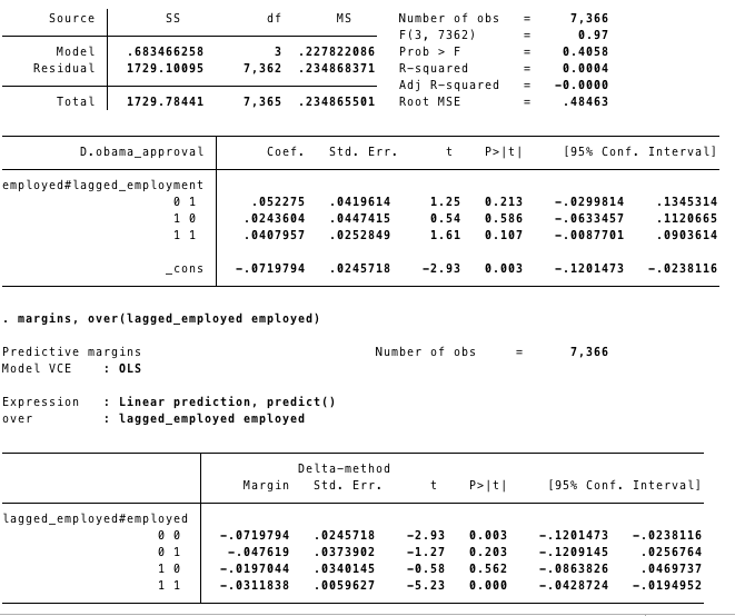
reg d1.obama_approval lagged_employed#employed
margins, over(lagged_employed employed)
Using the margins command after the regression provides a very easy way of seeing how approval changes among each of the four groups. For example, there was a .07 point drop in approval among individuals who were unemployed in one time period and stayed unemployed in the next wave. By comparison, approval dropped .048 for those who moved from being unemployed to being employed. Given the size ot the standard errors for these means, there is no significant difference between the two groups. You can also compare people who had a job and lost it to those who had and kept a job. Again, there is no sigificant difference in approval for these groups.
The difference-in-difference approach is often not the most efficient estimation of the data. This is because it only uses information comparing one time period to the period immediately before it; however, we can also learn something from comparing across multiple time periods. Additionally, the difference-in-difference approach works with binary treatment variables, but it does not easily handle variables with gradations (i.e. income, partisanship, etc.).
Another approach is using panel regression with unit fixed effects. To do this in Stata, we take advantage of the xtreg command.
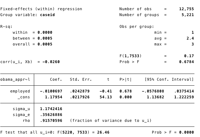
xtreg obama_approval employed, fe
The , fe options specifies a fixed effects model. Essentially, we are controlling for any time-invariant differences across individuals by taking this approach. The information being used to determine the effect of employment status on approval is only for individuals whose employment status changed at some point during the 3 waves. Based on this approach, employment status appears to be unrelated to approval for Obama (based on the coefficient for the employed variable).