Chapter 9 Survey Experiments
In this section we will learn about the strengths and weaknesses of survey experiments. We will then learn best practices for designing and analyzing such experiments.
The great thing about running an experiment is that analyzing the results is often pretty straightforward. I have a couple of basic “go-to” routines to present basic experimental treatment effects, which I’ll outline here. Of course, things can get increasingly complicated with experiments that have lots of conditions or other features, but this will get you started.
Here is a description of the experiment we’ll analyze here. It is a brief vignette, with random assignment of whether respondents received some kind of additional information about the candidate:
In Illinois, Democrat David Gill is running for a seat in the U.S. House of Representatives. Gill is an ER physician who is married and has six children with his wife Elaine. [RANDOMIZED TEXT HERE] He stated that he was running for Congress, “to revive the fading American Dream and make sure DC is setting the right priorities for our families again.”
Randomized text (with equal probability):
- No additional text (control condition).
- Gill was endorsed by the National Organization for Women.
- Gill was endorsed by the National Organization for Women because of his pro-choice views.
UMA311: Based on what you have heard, where would you place Gill on the ideological scale?
- Very liberal
- Liberal
- Somewhat liberal
- Moderate
- Somewhat conservative
- Conservative
- Very Conservative
The data to analyze this data can be accessed here.
Essentially, the idea was to see whether an endorsement from the National Organization for Women would change how liberal or conservative people thought the candidate was. So our key dependent variable is UMA311 – where respondents placed Gill on the 7-point ideological scale. And we want to see whether this varies across our three conditions (the control and 2 treatment conditions). A common way that people sometimes plot these things is just to show the overall level of the dependent variable for each condition. Something like this:
graph bar UMA311, over(condition)Of course, there are several problems with this particular graph. One is that we don’t have any uncertainty estimates for these figures (e.g. confidence intervals). We could recover this information by using a very basic regress command and then using marginsplot as so:
reg UMA311 i.condition
margins, over(condition)
marginsplot, recast(bar) xlabel(, angle(45)) title(" ") ytitle("Conservatism") xtitle(" ")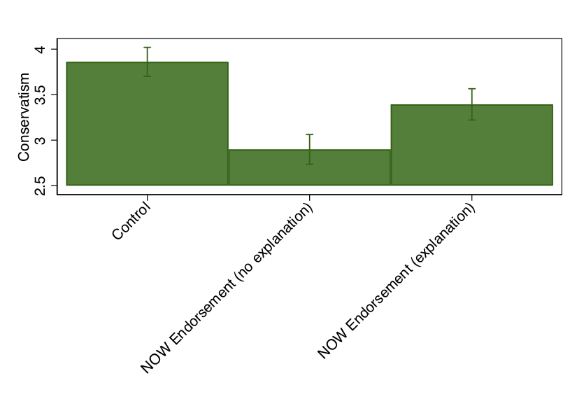
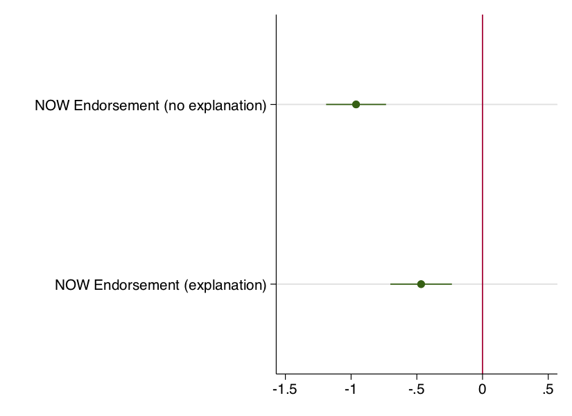
So this is a little better, and we could further play with this graph to clean this up. But it still isn’t as informative as we might prefer. In particular, what we really want here are the treatment effects. That is, the difference between the treatment condition(s) and the control condition. This graphic makes it so we have to figure that out for ourselves. So, a better approach would be to essentially produce a coefficient plot. There are a couple of ways to do this in Stata (including the margins command), but the easiest is to use the coefplot package.
reg UMA311 i.condition
coefplot, drop(_cons) xline(0) plotr(lc(none)) xlabel(-1.5 -1 -.5 0 .5)
A few points here. First, I use the drop(_cons) option to omit the plotting of the intercept. That is pretty much irrelevant to understanding the treatment effects and it is confusing to have it in the same plot.
I like plotting a line at 0 (xline(0)) as a reference. If a treatment effect is significant, then the confidence interval for that effect should not overlap with the zero line. That is what we see here. This also gives us a better sense of the size of the treatment effects. The endorsement with no explanation moves peoples’ estimates of Gill’s ideology a full point more liberal, whereas the endorsement with the explanation only has an effect that is about half has large. Note that I had to use the xlabel(-1.5 -1 -.5 0 .5) option so that the reference line would show up since the default range for this particular plot would not include zero otherwise.
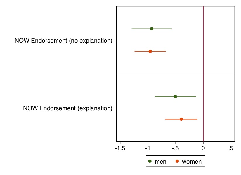
Finally, what if we want to see whether our treatment effects are heterogeneous by some other variable in our model? Well, the easiest thing to do is to estimate separate regression models and combine them into a single plot. In the code below, I estimate treatment effects for men, store the results, then for women (and store those results), and then use coefplot to bring in the results for both men and women into a single plot.
reg UMA311 i.condition if gender==0
est store men
reg UMA311 i.condition if gender==1
est store women
coefplot men women, drop( cons) xline(0) xlabel(-1.5 -1 -.5 0 .5)